Case
Study III: Control of a Double-Pipe Heat Exchanger
| Carla Martín-Villalba | |
| Departamento de Informática y Automática, UNED | |
| Juan del Rosal 16, 28040 Madrid, Spain |
the flow paths of the water and the gas, and the pipe wall in control volumes. This approach allows for local variations in physical properties and heat transfer coefficients. The diagram of the JARA model is shown in Figure 1a (it has been represented using Dymola).
the open loop system (see Figure 1a), the system controlled using a PID (see Figure 1b) and the system controlled using a compensator (see Figure 1c).
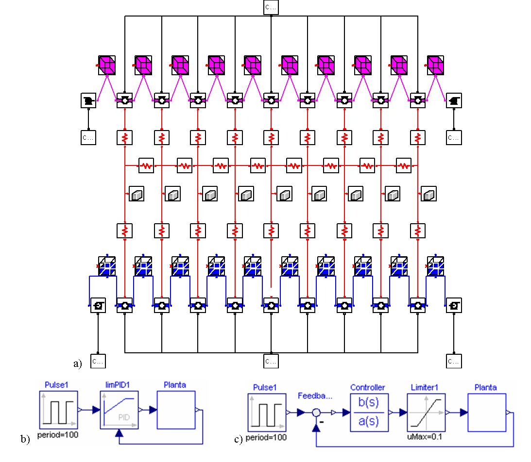
Figure 1: Diagram of the heat-exchanger
Modelica model: a) open-loop plant; b) plant controlled using a PID; and
c) plant controlled using a compensator.
In addition, a Sysquake application has been programmed. It implements the virtual-lab view and controls the execution of the Dymola executable files. The features of this Sysquake application, that constitutes the virtual-lab core, include:
| 1. | The application to the heat-exchanger model of several identification techniques. |
| 2. | The design of control strategies (using the linear models previously obtained by applying the identification techniques). |
| 1. | The change in the value of the gas exit temperature, in response to a step in the water flow, is calculated simulating the heat exchanger model |
| 2. | A transfer function (abbreviated: TF) is fitted to this response. |
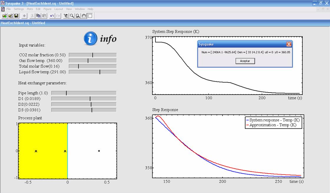
Figure 2: View of the double-pipe
heat-exchanger virtual-lab: plant linearization.
| 1. | Change the parameter values and the input variable values of the heat exchanger model, the simulation communication interval and the total simulation time. |
| 2. | Choose among different identification methods, including "first order TF with delay", "second order TF with delay" and "non-parametric identification". |
| 3. | Modify the obtained TF. |
| 4. | Analyze the obtained TF by means of Bode and zero-pole diagrams, and robustness margins. |
| 5. | Start the simulation run. |
| 6. | Export the calculated TF to another Sysquake application. |
| 1. | To import the TF previously identified. |
| 2. | To analyze the TF characteristics using Nyquist, Nichols and Bode diagrams. |
| 3. | To choose the controller type (possible options are: PID, lead and lag compensators). |
| 4. | To synthesize the controller (i.e., to set the value of the PID's parameters). |
| 5. | To specify the error and the phase margin of the system controlled by the lead or lag compensators. |
| 6. | To simulate the closed-loop linear and non-linear models. |
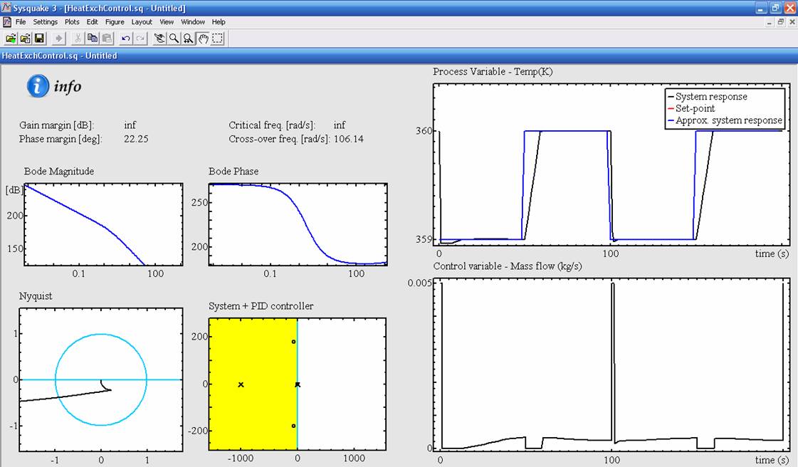
Figure 3: View of the double-pipe
heat-exchanger virtual-lab: controller synthesis.