| |
| |
|
|
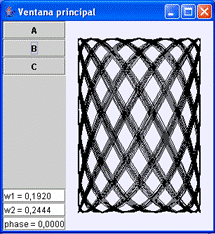
Fig.
7.1: View of the virtual-lab. |
|
|
|
|
|
| System
description |
| |
| Lissajous
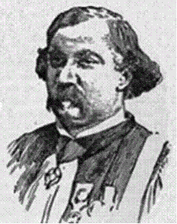
curves were studied by the French physicist and mathematician Jules Antoine
Lissajous (see Fig. 7.10). |
| |
|
Fig.
7.10: Jules Antoine Lissajous (1822-1880). |
| |
| Lissajous
curves are the composition of two harmonic motions (sinusoids): |
|
| |
The
curve shape,  ,
depends on the frequency ratio, ,
depends on the frequency ratio,  ,
and the phase, ,
and the phase,  . . |
| |
| This
virtual-lab enables to analyze the Lissajous figures. The view of the virtual-lab
contains three buttons (A, B and C), which set predefined values to the
frequency and the phase of the harmonic signals. In addition, the numerical
values of the frequency and the phase can be selected by the lab's user. |
|
|
| Introduction |
| |
| When
Ejs is launched, the Introduction panel is selected (see Fig. 7.11). Click
on the panel to create a new Introduction page. |
| |
|
Fig.
7.11: Initial window of Ejs. |
| |
Once
the introduction page has been created, you can write text, insert images,
etc. The contents included in a Introduction page by the user are automatically
translated into HTML by Ejs. If you click on View (i.e., second
item of the menu bar) and select the Source check box, then the
HTML code is displayed. |
| |
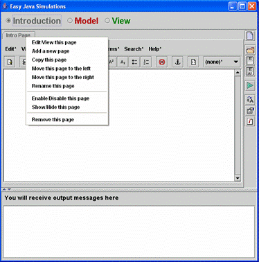
| Press
the right mouse button on the page tab to open the page menu (see Fig 7.12).
This menu allows to add, copy, move, and remove a Introduction page. |
| |
|
Fig.
7.12: Menu of the Introduction pages. |
| |
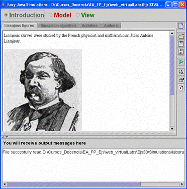
| The Introduction pages of the virtual-lab are shown in Fig 7.13. |
| |
|
Fig.
7.13: Introduction pages of the virtual-lab. |
| |
|
|
| Model |
| |
| The
model is composed of the two following equations: |
|
| |
The
amplitude, the frequencies and the phase are model parameters. The horizontal
( )
and vertical ( )
and vertical ( )
positions are unknown algebraic variables. The analysis of the computational
causality results in the following: )
positions are unknown algebraic variables. The analysis of the computational
causality results in the following: |
|
| |
| The
Ejs' simulation algorithm of this model is shown in Fig. 7.14. The maximo
and minimo variables
represent the maximum and minimum value of the oscilloscope’s display
range. The n variable
represents the number of points of the oscilloscope trace. These variables
are used for defining the virtual-lab view. The variable deltaTiempo
is the time step size. The tiempo
variable is the simulated time. |
| |
|
Fig.
7.14: Ejs' simulation algorithm of this model. |
| |
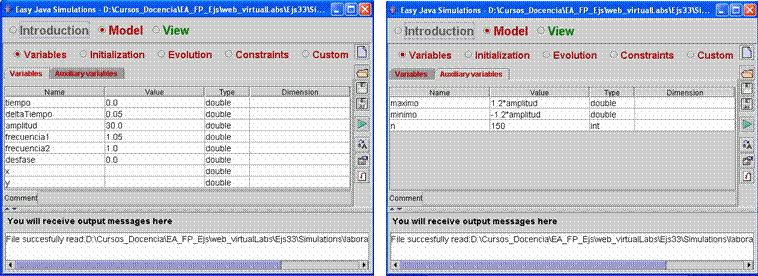
| The
content of the Variable panel is shown in Fig. 7.15. The variables have
been declared using two pages: “Variables” (which contains the
variables of the mathematical model) and Auxiliary variables (which contains
the variables used in the view). |
| |
|
Fig.
7.15: Declaration of the model variables. |
| |
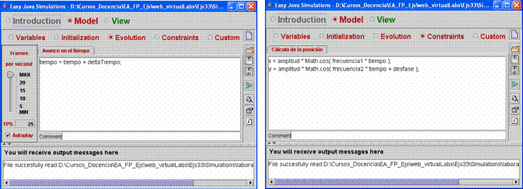
| The
contents of the Evolution and Constraints panels are shown in Fig. 7.16.
|
| |
|
Fig.
7.16: Evolution and Constraints panels. |
|
|
| View |
| |
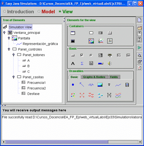
| The
tree of elements is shown in Fig. 7.17. Open the virtual-lab (lissajous_en.xml)
and look at the properties of the tree elements. Press the mouse right button
on a node to display its properties. |
| |
|
Fig.
7.17: Tree of elements. |
|
