| |
Case
Study IV: Control of an Industrial Boiler |
| |
| Author |
| |
Carla
Martín-Villalba |
| |
Departamento
de Informática y Automática, UNED |
| |
Juan del Rosal
16, 28040 Madrid, Spain |
|
|
|
| |
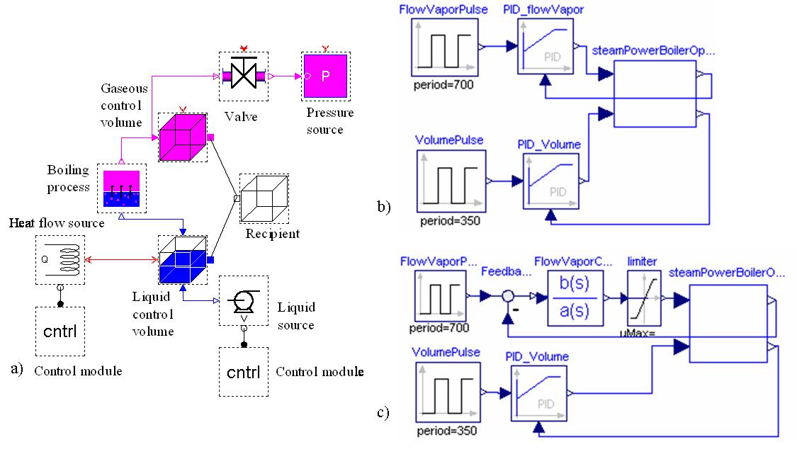
| The JARA Modelica
library has been used to compose the interactive model of an industrial
boiler. It is based on the mathematical model of the process provided in
(Ramirez 89). The model diagram is shown in Figure 1a (it has been represented
using Dymola). The input of liquid water is located at the boiler bottom,
and the vapor output valve is placed at the boiler top. The water contained
inside the boiler is continually heated. |
| |
|
Figure
1: Diagram of the boiler Modelica model composed using JARA. |
| |
| The model is composed
of two control volumes, in which the mass and energy balances are formulated:
(1) a control volume containing the liquid water stored in the boiler; and
(2) a control volume containing the generated vapor. The model of the boiling
process connects both control volumes. The heat flow from the heater to
the water, the pressure at the valve output and the water pump are modeled
using JARA source models. |
| |
| This virtual-lab is
intended to illustrate the indentification of the industrial boiler and
the synthesis of the boiler control system. This control system is composed
of two decoupled control loops: (1) the water level inside the boiler is
controlled by manipulating the pump throughput; and (2) the output flow
of vapor is controlled by manipulating the heater power. The identification
and synthesis procedures are similar to the one discussed in the Case
Study III. |
| |
| Three different Modelica
models has been built to identificate and control the system: the open loop
system (see Figure1a), the system controlled using two PIDs (see Figure
1b) and using a PID to control the water level inside the boiler and a compensator
to control the output flow of vapor (see Figure 1c). |
| |
| The identification
and synthesis procedures are briefly described next. The user is allowed
to choose interactively the plant's operation point. This is accomplished
by setting the value of: |
| - |
The
mass and temperature of the liquid and the vapor inside the boiler. |
| - |
The valve opening
and its downstream pressure. |
| - |
The flow and
inlet temperature of the water. |
|
| |
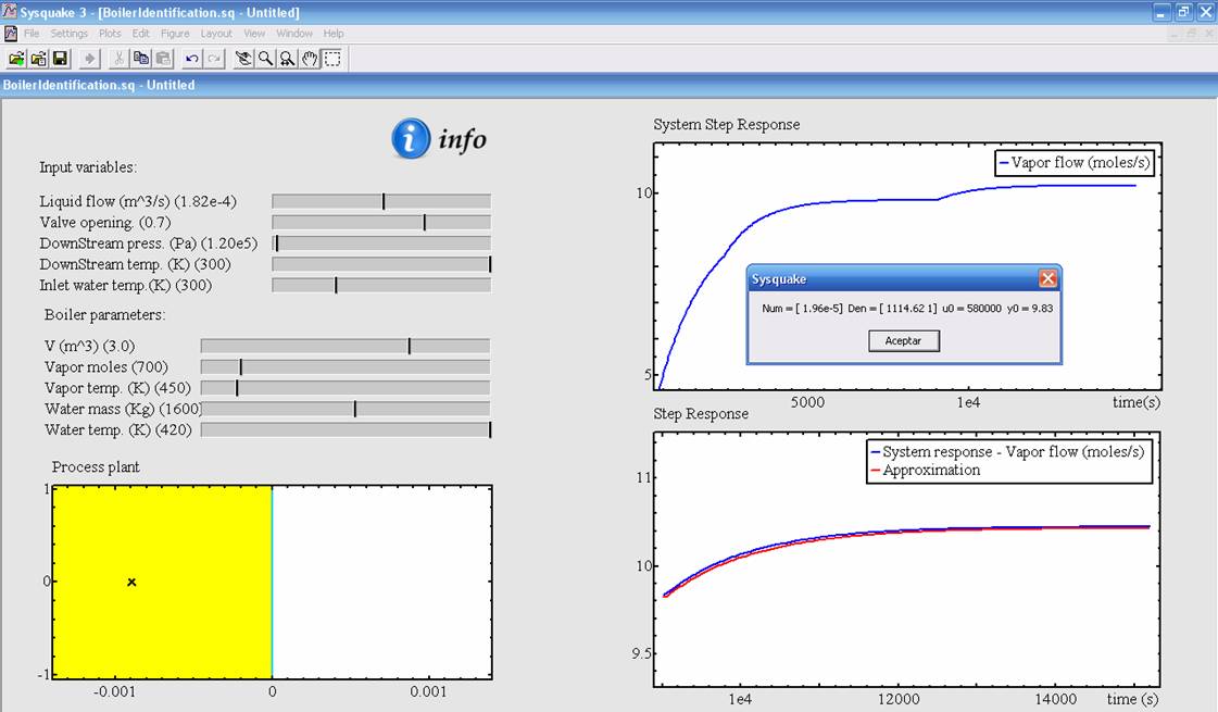
| Once the operation
point has been set, the user can launch the calculation of the two TF: (1)
a TF from the "pump throughput" (input) to the "water
level" (output); and (2) a TF from the "heater power"
(input) to the "vapor flow" (output). These TF are automatically
fitted to simulated step responses by the virtual-lab. The user can choose
among the following identification methods (see Figure2): "first
order TF with delay", "second order TF with delay"
and "non-parametric identification". |
| |
|
Figure
2: View of the boiler virtual-lab: plant linearization. |
| |
| The virtual-lab supports
a set of graphical methods to analyze the fitted TF, including Bode and
pole-zero diagrams, and it automatically computes the robustness margin.
In addition, the virtual-lab allows to export the TF to any other Sysquake
application. |
| |
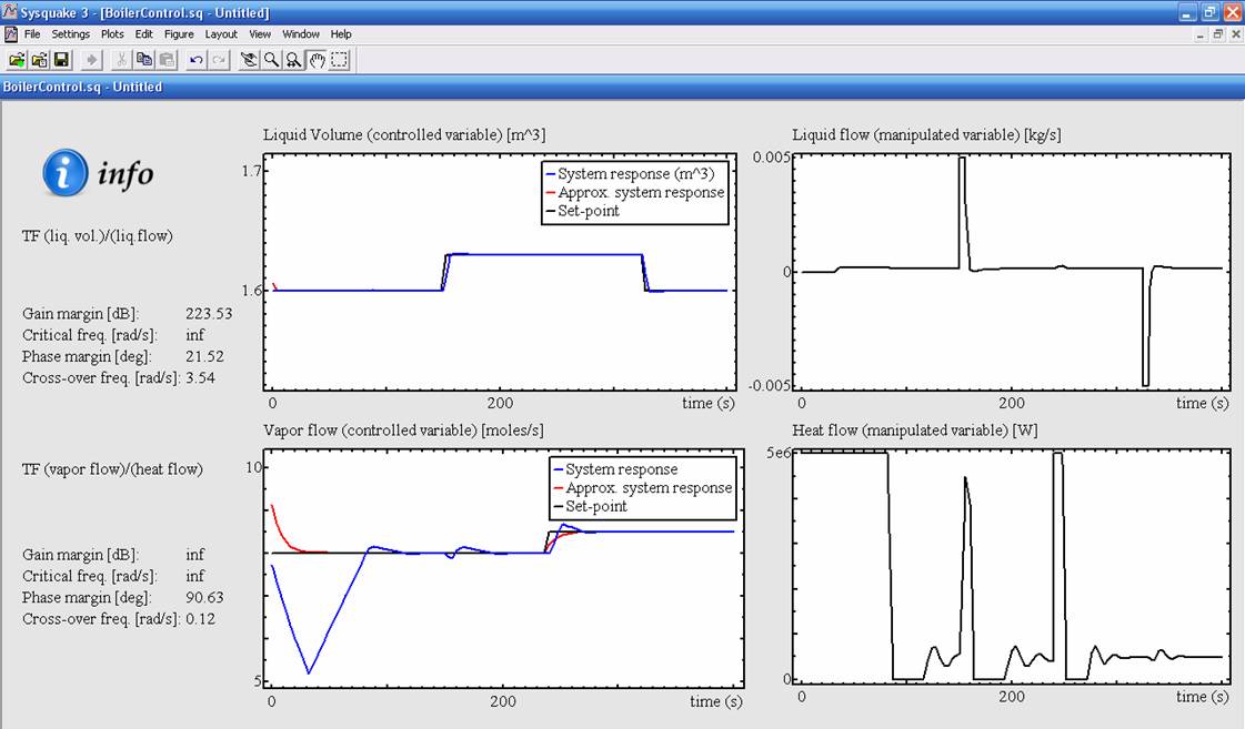
| Finally, the virtual-lab
facilitates the design and analysis of the two controllers (see Figure3).
The water level inside the boiler is controlled using a PID. The gas flow
can be controlled using a PID, a lead or a lag compensator. The user can
change the controller parameters, and the error and phase-margin specifications
of the compensation networks. |
| |
|
Figure
3: View of the boiler virtual-lab: controller synthesis. |
| |
| An experience using
the industrial boiler virtual-lab will be described below. The following
TF has been considered to describe the changes in the liquid levels due
to changes in the pump flow: 1.3/s. A change in value of the heat flow from
5.8E5 W to 6.0E5 W has been applied to the heat exchanger at time 9000 s.
The operation conditions of the boiler are shown in Figure 2. A TF has been
fitted to the vapor flow by applying a first order identification method.
The following TF has been obtained: |
|
| |
| Two PID controllers
have been designed. The PID that controls the liquid volume inside the boiler
has the following parameters: |
Kp
= 1, Ti = 9, Td = 1E-3, wp = 1, wd = 1, Ni = 0.9, Nd = 10, ymin = -0.01,
ymax = 0.01 |
| The PID that controls
the vapor output flow has the following parameters: |
Kp
= 7E6, Ti = 1.1, Td = 3E-3, wp = 1, wd = 1, Ni = 0.9, N_d = 10, ymin =
0, ymax = 5E6. |
| The time evolution
of the set-points, the manipulated variables and the control variables are
shown in Figure 3. |
| |
| References |
| W. F. Ramirez (1989):
"Computational Methods for Process Simulation", Butterworths
Publishers, Boston, USA. |
| |
|
| Carla Martin-Villalba |
| Last update: July
2007 |
| euclides
web server - Dept. Informatica y Automatica, UNED, Juan del Rosal 16,
28040 Madrid, Spain |